
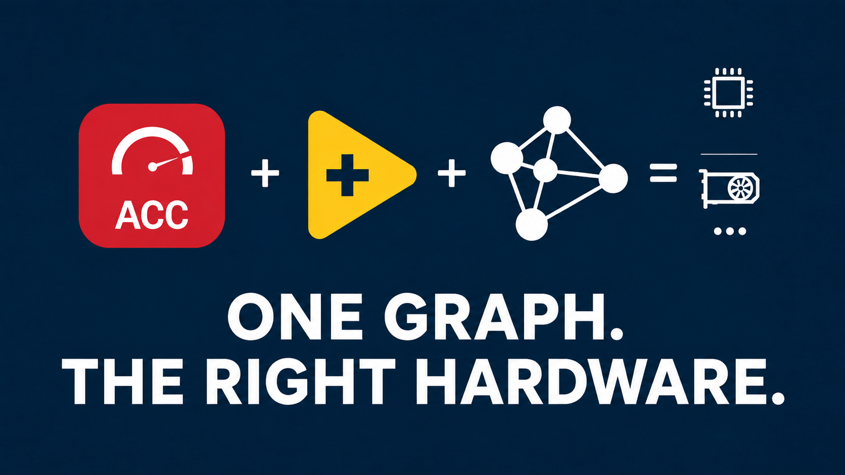
Adding a GPU to a LabVIEW system does not automatically make the application faster. Real acceleration appears when the workload is large enough, data movement is controlled, and the complete computation pipeline can be optimized instead of being executed as a succession of isolated function calls.
This is where ONNX Runtime Execution Providers become important. They separate the computation graph from the hardware-specific execution strategy, allowing the same ONNX graph to run on CPUs, NVIDIA GPUs, Intel hardware, Windows-compatible GPUs, NPUs, and other accelerators through a consistent runtime interface.
Graiphic brings this architecture into LabVIEW through the LabVIEW Accelerator Toolkit. The objective is not simply to call CUDA functions from a block diagram. It is to use LabVIEW as a graphical environment for building, configuring, and executing optimized ONNX computation graphs.
The key idea is simple: the objective is not to execute every function on the GPU. It is to execute every part of the graph on the architecture that processes it best.
Why a GPU Does Not Automatically Make LabVIEW Faster
A GPU is designed for throughput. It becomes highly effective when thousands of similar operations can be executed in parallel, as in matrix multiplication, FFT processing, image operations, tensor transformations, and neural-network inference.
However, the total time observed by LabVIEW includes more than the mathematical calculation itself:
Total latency = preparation + CPU-to-device transfer + kernel launch + computation + device-to-CPU transfer + synchronization.
For a large matrix multiplication, computation can dominate this equation and the GPU can provide a major advantage. For a small array operation, the transfer and launch overheads may cost more than the calculation. In that case, a modern CPU may remain faster.
This is why a meaningful benchmark must distinguish session initialization, warm-up, data transfers, stabilized execution time, and end-to-end application latency. A fast kernel does not necessarily produce a fast system.
NI describes CPUs, FPGAs, and GPUs as complementary processing resources: the CPU is well suited to orchestration and sequential logic, the FPGA to deterministic hardware-timed execution, and the GPU to highly parallel workloads such as signal processing, image analysis, and AI inference. The most efficient architecture is therefore often hybrid rather than GPU-only. The engineering implications are discussed in NI’s overview of GPU acceleration for LabVIEW test systems.
What Is an ONNX Runtime Execution Provider?
An Execution Provider, commonly abbreviated as EP, is the hardware abstraction layer used by ONNX Runtime to connect an ONNX graph to a hardware-specific execution library.
It is not simply a device driver. A CUDA driver allows software to communicate with an NVIDIA GPU. The CUDA Execution Provider tells ONNX Runtime which ONNX operators it can execute, how memory should be allocated, which optimized kernels should be used, and how computation should be scheduled on the device.
LabVIEW application
        ↓
LabVIEW Accelerator Toolkit
        ↓
ONNX computation graph
        ↓
ONNX Runtime
        ↓
Execution Provider
        ↓
CPU / CUDA / TensorRT / DirectML / OpenVINO / oneDNN
        ↓
Target processor, GPU, or accelerator
ONNX Runtime asks each registered provider which nodes or subgraphs it can execute. The runtime then partitions the graph and assigns compatible sections to the available providers. This mechanism allows the application to keep a stable interface while the deployment strategy changes.
Provider Priority, Partitioning, and Fallback
An ONNX Runtime session can register several providers in priority order. A common NVIDIA configuration is:
providers = [
    "TensorrtExecutionProvider",
    "CUDAExecutionProvider",
    "CPUExecutionProvider"
]
This does not guarantee that the complete graph will run with TensorRT. It means that TensorRT receives the first opportunity to claim compatible subgraphs, CUDA can execute remaining compatible nodes, and the CPU provider handles unsupported operations.
ONNX graph
    ├── TensorRT-compatible subgraph → TensorRT engine
    ├── Remaining GPU-compatible nodes → CUDA
    └── Unsupported accelerator nodes → CPU fallback
Fallback is useful because it can keep a graph executable, but it is not free. An unsupported operator in the middle of a GPU pipeline can introduce synchronization and memory transfers between the host and device. The application may run correctly while performing far below expectations.
This is why provider coverage must be verified at the node level. Graiphic created an open project to test ONNX operators across CPU, CUDA, TensorRT, OpenVINO, oneDNN, and DirectML, classifying results as success, fallback, failure, or not tested. The project is introduced in Graiphic’s ONNX Runtime Execution Provider coverage article.
What ONNX Runtime Does Before the First Execution
ONNX Runtime does not simply read one node after another and call a corresponding function. When a session is created, the runtime prepares the graph through several stages.
1. Graph validation
The runtime validates operator definitions, tensor types, attributes, input-output relationships, and available shape information.
2. Graph optimization
ONNX Runtime can perform constant folding, remove redundant nodes, eliminate unnecessary identities, fuse compatible operations, and optimize data layouts. These transformations reduce the amount of work performed at runtime and can expose larger regions for hardware acceleration. The available optimization levels are documented in the official ONNX Runtime graph optimization guide.
3. Graph partitioning
Each Execution Provider declares the nodes and subgraphs it supports. ONNX Runtime assigns graph sections according to provider priority and compatibility.
4. Hardware-specific preparation
Depending on the provider, this stage can include kernel selection, memory planning, layout conversion, subgraph compilation, or the construction of a hardware-specific execution engine. TensorRT can compile compatible subgraphs into optimized engines for the target NVIDIA GPU.
5. Memory planning
The runtime identifies tensor lifetimes, reusable buffers, allocator boundaries, and the points where data must cross between CPU and accelerator memory.
The preparation cost explains why a session should generally be created once, warmed up, and reused throughout the processing loop.
The Main Execution Providers Relevant to LabVIEW Workloads
| Execution Provider | Target | Main advantage | Main consideration |
|---|---|---|---|
| CPU | x86 or Arm CPU | Universal compatibility and low startup overhead | Lower throughput for large highly parallel workloads |
| oneDNN | Optimized Intel execution | Vectorized and multithreaded primitives | Benefits depend on the processor and operator coverage |
| CUDA | NVIDIA GPU | Broad GPU coverage and flexible acceleration | CUDA, cuDNN, memory transfer, and synchronization constraints |
| TensorRT | NVIDIA GPU and supported Jetson systems | Subgraph compilation, fusion, and precision optimization | Engine build time, tensor shapes, and unsupported operators |
| DirectML | DirectX 12-compatible Windows GPU | Cross-vendor Windows GPU deployment | Performance depends on hardware, driver, and graph coverage |
| OpenVINO | Intel CPU, GPU, and supported NPU | Deployment across the Intel hardware ecosystem | Device-specific compatibility and configuration |
There is no universally best provider. The correct choice depends on graph structure, data types, tensor dimensions, hardware availability, latency requirements, and the proportion of the graph that the provider can execute without fallback.
What the LabVIEW Accelerator Toolkit Changes
The LabVIEW Accelerator Toolkit uses ONNX as a general computation-graph representation and ONNX Runtime as the execution engine. Although ONNX is widely associated with AI model exchange, an ONNX graph fundamentally describes typed tensor operations connected by explicit data dependencies.
This makes it possible to represent more than neural-network inference. A graph can combine arithmetic, matrix multiplication, reductions, tensor transformations, signal-processing operations, custom operators, and AI models inside the same execution pipeline.
Graiphic introduced this approach to turn LabVIEW into a graphical environment for general-purpose ONNX graph computing. The design direction is presented in LabVIEW Evolves into a Graph Editor and in Graiphic’s broader 2025–2026 LabVIEW AI ecosystem overview.
GraphMX: Turning an ONNX Graph into a LabVIEW Component
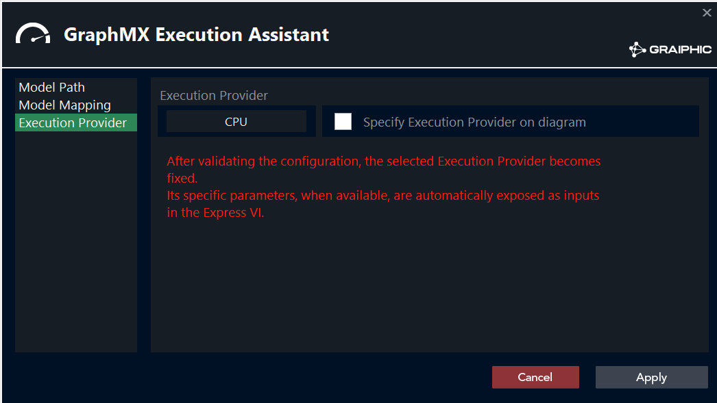
GraphMX is the Express VI used to configure an ONNX graph for execution from LabVIEW. It reads the model interface, maps inputs and outputs, configures the Execution Provider, and generates a VI that can be wired directly into the block diagram.
- Select an ONNX model or computation graph.
- Inspect its input and output names, types, and dimensions.
- Map ONNX tensors to LabVIEW terminals.
- Select a fixed Execution Provider or expose the provider as a diagram input.
- Configure provider-specific parameters when required.
- Generate a reusable execution VI without rebuilding the ONNX Runtime session interface manually.
This creates a clean separation between functional behavior and deployment:
One ONNX graph
    ├── Development workstation → CPU or DirectML
    ├── NVIDIA test station → CUDA
    ├── Optimized NVIDIA deployment → TensorRT + CUDA fallback
    └── Intel industrial computer → OpenVINO or oneDNN
The LabVIEW application can preserve the same high-level interface while the runtime configuration changes according to the target machine.
Why Full-Graph Execution Can Outperform Function-by-Function GPU Calls
Consider a simplified signal-processing chain:
Acquisition
    → offset correction
    → windowing
    → FFT
    → magnitude
    → logarithm
    → normalization
    → matrix multiplication
    → detection
In a traditional function-by-function architecture, each operation can cross a separate API or DLL boundary. Even if every individual function uses the GPU, the complete pipeline may repeatedly allocate memory, submit kernels, synchronize, and return control to LabVIEW.
LabVIEW → function DLL → LabVIEW → FFT DLL → LabVIEW → matrix DLL → LabVIEWEach function sees only its own inputs and outputs. It cannot necessarily determine that an intermediate result should remain on the GPU, that two operations could be fused, or that a buffer can be reused.
With a complete ONNX graph, ONNX Runtime and the selected provider can analyze the pipeline as a whole:
LabVIEW → complete ONNX graph → optimization → provider execution → resultThe runtime can remove redundant work, reuse buffers, retain intermediate tensors on the accelerator, select kernels according to tensor shapes, and compile compatible subgraphs. The hardware has not changed; the runtime simply has more information with which to optimize execution.
Memory Movement Is Often the Real Bottleneck
One of the most common GPU integration errors is to optimize the calculation while ignoring the cost of moving data.
LabVIEW array in system memory
        → CPU-to-GPU copy
        → graph execution
        → GPU-to-CPU copy
        → LabVIEW array
If this sequence occurs after every small operation, PCI Express transfers and synchronization can dominate the total duration.
ONNX Runtime provides I/O Binding so inputs and outputs can be associated with memory located on the target device before execution. This allows the runtime to avoid automatic copies inside each call.
A better high-throughput architecture is:
Acquisition
    → grouped transfer or device-resident buffer
    → preprocessing on the GPU
    → FFT, GEMM, filtering, or inference
    → post-processing on the GPU
    → compact result returned to LabVIEW
Instead of returning complete intermediate tensors, the system may return only a classification, an anomaly score, a target position, a reduced matrix, a decimated spectrum, or an alarm state.
What Graiphic’s Open GPU Benchmarks Show
Graiphic published the methods, LabVIEW sources, and results used to compare four execution approaches:
- LabVIEW Accelerator Toolkit, identified as Graiphic Accelerator in the benchmark.
- CuLab GPU Toolkit 4.1.2.80.
- G2CPU GPU and CPU HPC Toolkit 1.6.0.15.
- Native LabVIEW CPU execution.
The published test platform used Windows 11, an Intel Core i9-10850K, an NVIDIA GeForce RTX 3060, LabVIEW 2025 Q3, CUDA 12.8, TensorRT 10.13.3.9, and DirectML 1.15.4.0. The complete project is available in the open LabVIEW GPU Benchmarks repository.
Benchmarked workloads
- GEMM: matrix multiplication followed by arithmetic post-processing.
- Arithmetic graph: repeated Add, Negate, Multiply, and Divide operations.
- Complex-number computation: real and imaginary tensor processing through custom ONNX paths.
- Signal processing: FFT and arithmetic operations on realistic signal blocks of approximately 32,000 samples.
In that specific hardware and software configuration, the TensorRT path reached differences of up to 5× compared with CuLab and 40× compared with G2CPU. These figures are maximum results from the published scenarios, not universal ratios for every computer and every algorithm.
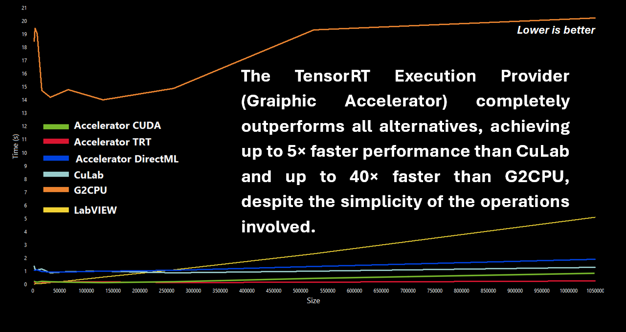
The results also show why workload size matters. The CPU remains competitive on smaller blocks because it avoids device-transfer and kernel-launch costs. GPU benefits increase as the amount of parallel computation grows and as more operations remain inside one coherent graph.
How to interpret the benchmark correctly
Performance can change with matrix dimensions, tensor shapes, numerical precision, GPU architecture, PCI Express bandwidth, driver versions, provider coverage, session reuse, warm-up strategy, and memory management. The most important contribution of the benchmark is therefore its reproducibility: engineers can inspect and rerun the same LabVIEW code on their own hardware.
Worked Example: Local Multi-Channel Sensor Processing
Consider an illustrative aerospace or defense test platform acquiring synchronized complex I/Q data. The processing must remain local because the raw data is sensitive, network bandwidth is limited, and the decision latency must remain low.
Assume the system acquires:
- 32 complex I/Q channels;
- 50 million samples per second per channel;
- 16 bits for I and 16 bits for Q;
- 4 bytes per complex sample.
The raw data rate is:
32 × 50,000,000 × 4 bytes = 6.4 GB/s, or approximately 51.2 Gbit/s.
This figure excludes timestamps, packet headers, redundancy, metadata, and additional sensors. Sending the complete raw stream continuously to a remote server would be expensive and may be impossible in a disconnected or contested environment.
NATO’s 2026 Alliance Digital Strategy explicitly identifies tactical-edge computing, low-latency connectivity, local inference, sensor-data fusion, and operational autonomy in degraded or denied environments as strategic requirements.
The cost of a covariance calculation
A common multi-channel operation is the covariance matrix:
R = X × XH / N
For 32 channels, the result contains 32 × 32 = 1,024 complex coefficients. A direct full-matrix update at 50 million sample vectors per second represents approximately:
32² × 50,000,000 = 51.2 billion complex multiply-accumulates per second.
Using an approximate cost of eight real floating-point operations per complex multiply-accumulate gives an order of magnitude of:
51.2 billion × 8 ≈ 409.6 billion operations per second, or approximately 0.41 TFLOP/s.
This estimate does not yet include gain and phase correction, windowing, FFTs, filtering, correlations, classification, AI inference, or visualization. A processing chain that appears conventional can therefore become too expensive for sequential CPU execution.
A Practical Hybrid Architecture
Converters and acquisition hardware
                ↓
FPGA or hardware-timed acquisition
  triggering, synchronization, alignment, DMA
                ↓
Acquisition buffers
                ↓
GPU through the LabVIEW Accelerator Toolkit
  FFT, filtering, GEMM, covariance, inference
                ↓
Reduced results
  events, scores, spectra, matrices, alarms
                ↓
LabVIEW application
  orchestration, display, logging, communications
The FPGA handles deterministic acquisition and timing. The CPU manages state, sequencing, communications, safety logic, and the user interface. The GPU performs high-throughput parallel computation. The Execution Provider maps the graph to the installed accelerator.
Instead of transmitting 6.4 GB/s of raw information, the platform can transmit compact results such as detected events, confidence scores, feature vectors, reduced spectra, or health indicators.
Intelligent Use Cases Beyond Neural-Network Inference
RF and signal analysis
- Multi-channel FFT and spectrogram generation.
- Cross-correlation and covariance calculation.
- Channelization and interference analysis.
- Matrix-based sensor fusion.
- Signal anomaly detection and classification.
Visible and infrared vision
- Sensor correction, resizing, normalization, and fusion.
- AI inference followed by geometric and temporal post-processing.
- Keeping image buffers on the GPU from acquisition to final result.
Hardware-in-the-loop and simulation
- Large matrix-based plant models.
- Parallel scenario evaluation.
- Monte Carlo simulation.
- State estimation and observer calculations.
- Batch comparison of control configurations.
Predictive maintenance
Vibration acquisition
    → filtering
    → STFT or spectrogram
    → feature extraction
    → model execution
    → anomaly score
Local processing can reduce storage by retaining only relevant windows instead of recording every raw sample indefinitely.
Scientific, medical, and industrial imaging
- Multidimensional reconstruction.
- Denoising and registration.
- Segmentation and volumetric processing.
- Matrix transformations and accelerated inference.
Energy and critical infrastructure
- State estimation and transient analysis.
- Large time-series processing.
- Local event detection.
- Scenario simulation where cloud connectivity cannot be assumed.
When the GPU Is Not the Correct Choice
CPU execution may remain preferable when tensors are small, the calculation is infrequent, the graph contains irregular branches, data must return to LabVIEW after every operation, tensor shapes change constantly, or most operations fall back to the CPU.
An FPGA remains preferable when the requirement is cycle-accurate deterministic timing, custom digital protocols, fixed trigger latency, or hard real-time I/O behavior.
The GPU should be treated primarily as a throughput engine. Under a general-purpose Windows environment, it should not automatically be considered a hard real-time processor.
Ten Rules for Effective Acceleration
- Create the ONNX Runtime session once. Open it before the main processing loop and reuse it.
- Warm up the graph. Exclude first-run allocation, kernel selection, and TensorRT engine construction from stabilized measurements.
- Measure end-to-end latency. Include transfers, synchronization, and LabVIEW integration rather than timing only the kernel.
- Keep data on the accelerator. Use device-resident buffers and I/O Binding when several accelerated stages are chained together.
- Inspect provider assignment. A successful run may still contain expensive CPU fallback.
- Prefer coherent graphs. Larger compatible subgraphs provide more optimization opportunities than many disconnected calls.
- Stabilize tensor shapes when possible. Fixed or bounded dimensions help memory planning, kernel selection, and TensorRT compilation.
- Reuse TensorRT caches. Engine and timing caches can reduce deployment startup costs.
- Choose the correct batch size. Balance throughput against application latency.
- Benchmark on the target machine. Performance depends on the complete hardware, software, and memory architecture.
Conclusion
An Execution Provider is not simply a menu option that switches between CPU and GPU. It is the hardware abstraction layer that tells ONNX Runtime which parts of a graph can be accelerated, how they should be partitioned, where memory should be allocated, and which optimized execution engine should run them.
The LabVIEW Accelerator Toolkit brings this architecture into graphical engineering workflows. A developer can represent a computation as an ONNX graph, configure its inputs and outputs through GraphMX, select the deployment provider, and execute it from LabVIEW without rebuilding a custom hardware interface for every project.
The largest improvements come from four architectural decisions:
- Give the runtime visibility over the complete pipeline.
- Reduce boundaries between individual operations.
- Keep intermediate data on the accelerator.
- Assign each part of the graph to the processor that handles it best.
The GPU is not the architecture. The computation graph, memory strategy, and Execution Provider together define the architecture.
Explore the Technology
- Discover the LabVIEW Accelerator Toolkit documentation.
- Review and reproduce the open LabVIEW GPU benchmarks.
- Read the official ONNX Runtime Execution Provider documentation.
- Explore the complete Graiphic SOTA ecosystem.